5. Examples

To find a curve of degree at most 2 such that $P(-1) = (1,0)$, $P(0) = (0,0)$, and $P(1) = (0,1)$:

We have $n = 2$, $t_0 = -1, t_1 = 0, t_2 = 1$.

$p_0 (t) = {\frac{\displaystyle (t-0)(t-1)}{\displaystyle (-1-0)(-1-1)}} = {\frac 1 2} (t^2 - t)$

$p_1 (t) = {\frac{\displaystyle (t-(-1))(t-1)}{\displaystyle (0-(-1))(0-1)}} = -(t^2 - 1)$

$p_2 (t) = {\frac{\displaystyle (t-(-1))(t - 0)}{\displaystyle (1-(-1))(1-0)}} = {\frac 1 2} (t^2 + t)$

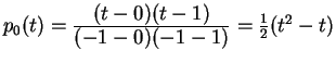
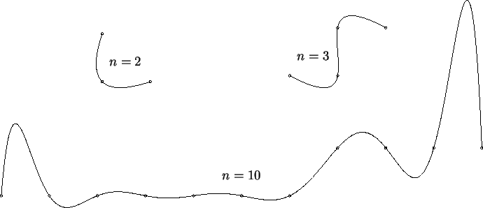
$P(t) = \frac 1 2(t^2 - t)(1,0) - (t^2 - 1)(0,0) + \frac 1 2(t^2 + t)(0,1) = ( \frac 1 2(t^2 - t), {\frac 1 2} (t^2 + t))$, as shown in the diagram.

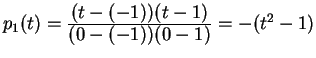
Figure shows this and two other examples.

Figure: Additional examples

In the lower example with $n = 10$, observe that the function is so wavy that it doesn't follow the data points very well. This is a disadvantage of working with polynomial functions of higher degrees. Moreover, by the uniqueness property (Theorem ) there is no other polynomial curve that has degree at most 10 and fits the data points.