5. Some applications

1. Making a loop: Use a Bézier curve in which the first and last control points coincide, as in Figure .

   Figure: Loops

   book/08dir/loop.eps

2. Making an arc: Just use these control points or similar ones, depending on the shape you want, as in Figure .

   Figure: Arcs

   book/08dir/arc.eps

   The control points in this example are $(0,0)$, $(.25,.25)$, $(.75,.25)$, $(1,0)$. If you instead want an arc of this exact shape between other given points $Q_0$ and $Q_1$, find an affine matrix that does a rotation, uniform scaling, and translation to move the segment $\overline {(0,0) (1,0)}$ to $\overline {Q_0 Q_1}$. To do this, write $Q_0 = (c,d)$ and $(a,b) = Q_1 - Q_0$ and then use the extended matrix ${\left[\begin{array}{rrr}a&b&0\\ -b&a&0\\ c&d&1\end{array}\right]}$.

   
   
   

3. Making a curved arrow: Add an arrowhead to a curved arc. For the arc in Figure , a suitable arrowhead goes from $(.95,0)$ to $(1,0)$ to $(1,.05)$. For a curved arrow with similar shape in a different position, apply an affine transformation as above. See Figure .

   Figure: A curved arrow

   book/08dir/arrow.eps

4. Making an S-curve: Just use a control polygon of the kind shown in Figure . Adjust as desired. If you add an arrowhead you could use such a curve in a flow chart to show a path from a box on one level to a box on a lower level.

   Figure: An S-curve

   book/08dir/scurve.eps

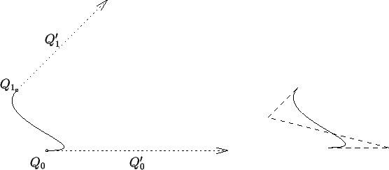
5. Hermite data: Suppose you want to find a cubic curve $Q(t)$ that has given values of $Q(0)$, $Q(1)$, $Q'(0)$, and $Q'(1)$. Let's call these values $Q_0$, $Q_1$, $Q'_0$, and $Q'_1$, respectively. They represent the initial and final positions and velocity vectors, as indicated in the left diagram below. This kind of problem is called an Hermite (``air-meet'') problem, after the French mathematician Hermite. There is exactly one solution.

   A solution is to use a Bézier curve with appropriate control points $P_0$, $P_1$, $P_2$, $P_3$. As you see, $P_0$ $=$ $Q_0$ and $P_3$ $=$ $Q_1$. Also, from the first derivative property, $3(P_1 - P_0)$ $=$ $Q'_0$ and $3(P_3 - P_2)$ $=$ $Q'_1$. These last two equations can be solved for $P_1$ and $P_2$. We get these Bézier control points, as shown in the right-hand portion of Figure .

   $$\begin{array}{ccc} P_0&=&Q_0\\ P_1&=&Q_0+{\frac 13} Q'_0\\ P_2&=&Q_1-{\frac 13} Q'_1\\ P_3&=&Q_1 \end{array}$$

   Figure: Hermite data