Homework 2

Table of Contents

Problem 1

Let X1,,XnX_1, \ldots, X_n be i.i.d. random variables with Poisson distribution with parameter λ\lambda. Find the maximum likelihood estimator for λ\lambda.

Solution.

The log-likelihood function is

lnL(θ)=lni=1nλxixi!eλ=i=1nxilnλi=1nln(xi!)nλ=nxlnλi=1nln(xi!)nλ\begin{aligned} \ln L\p{\theta} &= \ln \prod_{i=1}^n \frac{\lambda^{x_i}}{x_i!} e^{-\lambda} \\ &= \sum_{i=1}^n x_i \ln\lambda - \sum_{i=1}^n \ln\p{x_i!} - n\lambda \\ &= n\mean{x} \ln\lambda - \sum_{i=1}^n \ln\p{x_i!} - n\lambda \\ \end{aligned}

To optimize, we take the derivative with respect to λ\lambda and set it equal to 00 to get

lnL(θ)θ=nxλn=0    λ^=X.\begin{gathered} \frac{\partial \ln L\p{\theta}}{\partial \theta} = \frac{n\mean{x}}{\lambda} - n = 0 \\ \implies \boxed{\widehat{\lambda} = \mean{X}}. \end{gathered}

Problem 2

You throw a fair coin 3030 times. You observe that 55 times it lands on heads, and 2525 times it lands on tails. What is the maximum likelihood estimate for the probability that a single coin toss gives you heads?

Solution.

The MLE for a Bernoulli trial is p^=X\widehat{p} = \mean{X}, where Xi=1X_i = 1 if the coin lands on heads and 00 otherwise. In our case, we have the observed value X=530=16\mean{X} = \frac{5}{30} = \frac{1}{6}, so

p^=16.\boxed{\widehat{p} = \frac{1}{6}}.

Problem 3

Let y>0y > 0, θ>1\theta > 1. Define

f(x|y,θ)=θyθxθ1,xy.f\p{x \given y, \theta} = \theta y^\theta x^{-\theta-1}, \quad x \geq y.
  1. Show that f(x|y,θ)f\p{x \given y, \theta} is a probability density function.
  2. Assume that y>0y > 0 is given. Let X1,,XnX_1, \ldots, X_n be i.i.d. random variables with probability density function f(x|y,θ)f\p{x \given y, \theta}. Find the maximum likelihood estimator for θ\theta.
Solution.
  1. We just integrate with respect to xx:

    yθyθxθ1dx=θyθyxθ1dx=θyθxθθy=θyθ(0yθθ)=1.\begin{aligned} \int_y^\infty \theta y^\theta x^{-\theta-1} \,\diff{x} &= \theta y^\theta \int_y^\infty x^{-\theta-1} \,\diff{x} \\ &= \theta y^\theta \left. \frac{x^{-\theta}}{-\theta} \right\rvert_y^\infty \\ &= \theta y^\theta \p{0 - \frac{y^{-\theta}}{-\theta}} \\ &= 1. \end{aligned}

    Note that limxxθ=0\lim_{x\to\infty} x^{-\theta} = 0 since θ>0\theta > 0.

  2. The log-likelihood function is

    lnL(θ)=lni=1nθyθxiθ1=nlnθ+nθlny(θ+1)i=1nlnxi.\begin{aligned} \ln L\p{\theta} &= \ln \prod_{i=1}^n \theta y^\theta x_i^{-\theta-1} \\ &= n\ln\theta + n\theta \ln y - \p{\theta + 1} \sum_{i=1}^n \ln x_i. \end{aligned}

    Setting its derivative equal to 00, we get

    lnL(θ)θ=nθ+nlnyi=1nlnxi=0    θ^=11ni=1nlnXilny.\begin{gathered} \frac{\partial \ln L\p{\theta}}{\partial \theta} = \frac{n}{\theta} + n\ln y - \sum_{i=1}^n \ln x_i = 0 \\ \implies \boxed{\widehat{\theta} = \frac{1}{\frac{1}{n} \sum_{i=1}^n \ln X_i - \ln y}}. \end{gathered}

Problem 4

The midterm and final exam scores for 1010 students in a statistics course are tabulated as shown below.

Midterm62746630844514708242Final71847636955318809349\begin{array}{r|rrrrrrrrrr} \text{Midterm} & 62 & 74 & 66 & 30 & 84 & 45 & 14 & 70 & 82 & 42 \\ \text{Final} & 71 & 84 & 76 & 36 & 95 & 53 & 18 & 80 & 93 & 49 \end{array}
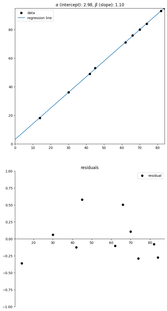
  1. Calculate the least squares regression line for these data.
  2. Plot the points and the least squares regression line on the same graph.
  3. Draw the residuals plot. What does this tell you?
  4. Find the maximum likelihood estimate for σ2\sigma^2.
Solution.

The least squares regression line is given by y=α^+β^xy = \widehat{\alpha} + \widehat{\beta} x with square residuals σ^2\widehat{\sigma}^2, where

α^2.98β^1.10σ^20.09\boxed{ \begin{aligned} \widehat{\alpha} &\approx 2.98 \\ \widehat{\beta} &\approx 1.10 \\ \widehat{\sigma}^2 &\approx 0.09 \end{aligned} }

The residuals are relatively small, so this is a good fit.

Python Code

I used numpy since it's faster to type (and runs faster), but you can do the computations without it if you don't want to. However, using numpy makes plotting with matplotlib a bit easier.

from matplotlib import pyplot as plt
import numpy as np

x = np.array([62, 74, 66, 30, 84, 45, 14, 70, 82, 42])
y = np.array([71, 84, 76, 36, 95, 53, 18, 80, 93, 49])

x_bar = np.mean(x)
y_bar = np.mean(y)

beta_hat = np.sum((y - y_bar) * (x - x_bar)) / np.sum((x - x_bar) ** 2)
alpha_hat = y_bar - beta_hat * x_bar
sigma2_hat = np.mean((y - alpha_hat - beta_hat * x) ** 2)

# Or without numpy:
# beta_hat = sum([(y[i] - y_bar) * (x[i] - x_bar) for i in range(n)]) / sum(
#     [(x[i] - x_bar) ** 2 for i in range(n)]
# )
# alpha_hat = y_bar - beta_hat * x_bar
# sigma_hat_2 = sum([y[i] - alpha_hat - beta_hat * x[i] for i in range(n)]) / n

print(f"alpha_hat:  {alpha_hat}")   # 2.9788895969084805
print(f"beta_hat:   {beta_hat}")    # 1.0987892865218194
print(f"sigma2_hat: {sigma2_hat}")  # 0.09218688976135175

fig = plt.figure(figsize=(8, 16))

# Plot sample and regression line
ax = fig.add_subplot(2, 1, 1)
ax.set_title(
    f"$\\alpha$ (intercept): {alpha_hat:>.2f}, $\\beta$ (slope): {beta_hat:>.2f}"
)
ax.set_xlim(0, np.max(x))
ax.set_ylim(0, np.max(y))
ax.scatter(x, y, c="black", label="sample")
ax.axline((0, alpha_hat), slope=beta_hat, label="regression line", zorder=-1)
ax.legend()

# Plot residuals
ax = fig.add_subplot(2, 1, 2)
ax.set_title("residuals")
ax.spines["top"].set_visible(False)
ax.spines["right"].set_visible(False)
ax.spines["bottom"].set_position("zero")
ax.set_ylim(-1, 1)
ax.set_yticks(np.linspace(-1, 1, 9))
ax.scatter(x, y - (alpha_hat + beta_hat * x), c="black", label="residual")
ax.legend()

Problem 5

For α>0\alpha > 0, β>0\beta > 0, the Beta distribution has probability density function

f(x|α,β)=Γ(α+β)Γ(α)Γ(β)xα1(1x)β1,x(0,1).f\p{x \given \alpha, \beta} = \frac{\Gamma\p{\alpha + \beta}}{\Gamma\p{\alpha} \Gamma\p{\beta}} x^{\alpha-1} \p{1 - x}^{\beta-1}, \quad x \in \p{0, 1}.

Find the method of moments estimator for α\alpha and β\beta.

Solution.

This is a straight calculation. The mean and variance of a Beta distribution are

E[X]=αα+β,VarX=αβ(α+β)2(α+β+1).\E\br{X} = \frac{\alpha}{\alpha + \beta}, \quad \Var X = \frac{\alpha\beta}{\p{\alpha + \beta}^2\p{\alpha + \beta + 1}}.

Note that

1ni=1n(xix)2=1ni=1nxi2+x2,\frac{1}{n} \sum_{i=1}^n \p{x_i - \mean{x}}^2 = \frac{1}{n} \sum_{i=1}^n x_i^2 + \mean{x}^2,

so when computing the method of moments estimator, we can just set

v=1ni=1n(xix)2=VarXv = \frac{1}{n} \sum_{i=1}^n \p{x_i - \mean{x}}^2 = \Var X

instead of using the second moment. This is only slightly easier, and the computations will be similar.

From the first moment,

x=α^α^+β^    β^=(1xx)α^andα^+β^=α^x,\mean{x} = \frac{\widehat{\alpha}}{\widehat{\alpha} + \widehat{\beta}} \implies \widehat{\beta} = \p{\frac{1 - \mean{x}}{\mean{x}}} \widehat{\alpha} \quad\text{and}\quad \widehat{\alpha} + \widehat{\beta} = \frac{\widehat{\alpha}}{\mean{x}},

which we can substitute into

v=α^β^(α^+β^)2(α^+β^+1)=(1xx)α^2(α^x)2(α^x+1)=(1x)xα^x+1    α^=((1x)xv1)x.\begin{aligned} v &= \frac{\widehat{\alpha}\widehat{\beta}}{\p{\widehat{\alpha} + \widehat{\beta}}^2\p{\widehat{\alpha} + \widehat{\beta} + 1}} \\ &= \frac{\p{\frac{1 - \mean{x}}{\mean{x}}} \widehat{\alpha}^2}{\p{\frac{\widehat{\alpha}}{\mean{x}}}^2\p{\frac{\widehat{\alpha}}{\mean{x}} + 1}} \\ &= \frac{\p{1 - \mean{x}}\mean{x}}{\frac{\widehat{\alpha}}{\mean{x}} + 1} \\ \implies \widehat{\alpha} &= \p{\frac{\p{1 - \mean{x}}\mean{x}}{v} - 1} \mean{x}. \end{aligned}

For β^\widehat{\beta},

β^=(1xx)α^=((1x)xv1)(1x)\widehat{\beta} = \p{\frac{1 - \mean{x}}{\mean{x}}} \widehat{\alpha} = \p{\frac{\p{1 - \mean{x}}\mean{x}}{v} - 1} \p{1 - \mean{x}}

so in summary,

α^=((1x)xv1)xβ^=((1x)xv1)(1x)\boxed{ \begin{aligned} \widehat{\alpha} &= \p{\frac{\p{1 - \mean{x}}\mean{x}}{v} - 1} \mean{x} \\ \widehat{\beta} &= \p{\frac{\p{1 - \mean{x}}\mean{x}}{v} - 1} \p{1 - \mean{x}} \end{aligned} }