<Home>Teaching><MATH 31B (Fall 2020)>Week 2 Discussion Notes

Week 2 Discussion Notes

Review of Exponentials and Logarithms
Differentiation and Integration
Logarithmic Differentiation
Homework

Review of Exponentials and Logarithms

Here are the main properties you'll want to remember:

Proposition

Let $b \in \p{0, \infty} \setminus \set{1}$ . Then

\begin{aligned} b^{x+y} &= b^xb^y &&& \log_b\p{xy} &= \log_bx + \log_by \\ \p{b^x}^k &= b^{kx} &&& \log_b\p{x^k} &= k\log_bx \\ b^0 &= 1 &&& \log_b1 &= 0 \end{aligned}

Notice how I arranged these equations—it's not a coincidence! On each row, the left and right equations are essentially the same. For example, in the first row, we turn a sum ( $x + y$ ) into a product ( $b^xb^y$ ) on the left and on the right, we turn a product ( $xy$ ) into a sum ( $\log_bx + \log_by$ ).

Example 1.

Assuming $b^{x+y} = b^xb^y$ is true, prove the identity $\log_b\p{xy} = \log_bx + \log_by$ for $x, y > 0$ .

Solution.

Since $x, y > 0$ , we can write $x = b^{\log_bx}$ and $y = b^{\log_by}$ . Then by assumption, $b^{\log_bx}b^{\log_by} = b^{\log_bx + \log_by}$ , so

\begin{aligned} \log_b\p{xy} &= \log_b\p{b^{\log_bx}b^{\log_by}} \\ &= \log_b\p{b^{\log_bx + \log_by}} \\ &= \log_bx + \log_by. \end{aligned}

Exercise 1.

Do the same thing for the last two identities from the proposition.

Another very important identity for logarithms is the change-of-base formula:

Theorem (change-of-base)

Let $a, b \in \p{0, \infty} \setminus \set{1}$ . Then

\log_ax = \frac{\log_bx}{\log_ba}.

Proof.

We can write $x = a^{\log_ax}$ , since logarithms and exponentials are inverses for the same base. Then

\log_bx = \log_b\p{a^{\log_ax}} = \p{\log_ax}\p{\log_ba}.

If we divide both sides by $\log_ba$ , we get the identity:

\log_ax = \frac{\log_bx}{\log_ba}.

$\square$

This is how I remember the formula: we're changing the base, so each side should use logarithms of only one base, i.e., in the formula, there are only $\log_a$ 's on the left side and only $\log_b$ 's on the right side.

To remember which one goes on top and which one goes on bottom, I like to use the fact that $a$ is written lower than $x$ ( $a$ is a subscript) on the left side. So, on the right side, $a$ should go on the "lower side," i.e., the denominator:

\log_{\colorbox{red}{$a$}}x = \frac{\log_bx}{\colorbox{red}{$\log_ba$}}.

Differentiation and Integration

Next, let's talk about the calculus of exponentials and logarithms. There are really only two things you need to remember:

\deriv{}{x} e^x = e^x \quad\text{and}\quad \deriv{}{x} \ln{x} = \frac{1}{x}.

This is because we have the formulas $b = e^{\ln{b}}$ and the change-of-base formula, and we'll see why right now.

Theorem

Let $b \in \p{0, \infty} \setminus \set{1}$ . Then

\deriv{}{x} b^x = b^x\ln{b} \quad\text{and}\quad \deriv{}{x} \log_bx = \frac{1}{x\ln{b}}.

Proof.

By the chain rule and the properties we talked about,

\deriv{}{x} b^x = \deriv{}{x} \p{e^{\ln{b}}}^x = \deriv{}{x} e^{x\ln{b}} = e^x\ln{b}.

Similarly, using the change-of-base formula, we get

\deriv{}{x} \log_bx = \deriv{}{x} \frac{\ln{x}}{\ln{b}} = \frac{1}{x\ln{b}}.

$\square$

Example 2.

Calculate $\int b^x \,\diff{x}$ .

Solution.

Let $u = b^x$ so that $\diff{u} = b^x\ln{b} \,\diff{x}$ . Then

\begin{aligned} \int b^x \,\diff{x} = \int \frac{b^x\ln{b}}{\ln{b}} \,\diff{x} &= \frac{1}{\ln{b}} \int \,\diff{u} \\ &= \frac{u}{\ln{b}} + C \\ &= \boxed{\frac{b^x}{\ln{b}} + C}. \end{aligned}

Example 3.

Calculate $\int \frac{\diff{x}}{x\ln{x}}$ .

Solution.

Let $u = \ln{x} \implies \diff{u} = \frac{1}{x} \,\diff{x}$ . The integral becomes

\int \frac{\diff{u}}{u} = \ln\abs{u} + C = \boxed{\ln{\abs{\ln{x}}} + C}.

Example 4.

Calculate $\int \frac{e^x - e^{-x}}{e^x + e^{-x}} \,\diff{x}$ .

Solution.

Let $u = e^x + e^{-x} \implies \diff{u} = \p{e^x - e^{-x}} \,\diff{u}$ . $u$ is precisely the denominator and $\diff{u}$ is the numerator, so the integral becomes

\int \frac{\diff{u}}{u} = \ln{\abs{u}} + C = \boxed{\ln{\abs{e^x + e^{-x}}} + C}.

Logarithmic Differentiation

The motivation behind this technique is that logarithms turn products into sums, and sums are much easier to work with than products. For example, try calculating the derivatives of $e^x + \sin{x}$ and $e^x\sin{x}$ . Which one was easier?

This technique is best illustrated through examples.

Example 5.

Calculate $\deriv{}{x} x^2e^x\sin{x}$ .

Solution.

When you want to use logarithmic differentiation, you always want to start by setting $y$ equal to what you want to take the derivative of. In this case, $y = x^2e^x\sin{x}$ , and if we take logarithms on both sides, we get

\begin{aligned} \ln{y} = \ln\p{x^2e^x\sin{x}} &= \ln\p{x^2} + \ln{e^x} + \ln\p{\sin{x}} \\ &= 2\ln{x} + x + \ln\p{\sin{x}}. \end{aligned}

Taking derivatives on both sides, we then get

\begin{aligned} \frac{y'}{y} = \frac{2}{x} + 1 + \frac{\cos{x}}{\sin{x}} &\implies y' = \p{\frac{2}{x} + 1 + \frac{\cos{x}}{\sin{x}}}y \\ &\implies y' = \boxed{\p{\frac{2}{x} + 1 + \cot{x}}x^2e^x\sin{x}}. \end{aligned}

Example 6.

Calculate $\deriv{}{x} e^{\sin{x}}\sqrt{\tan{x}}$ .

Solution.

Setting $y = e^{\sin{x}}\sqrt{\tan{x}}$ and taking logarithms as before,

\begin{aligned} \ln{y} = \ln\p{e^{\sin{x}}\sqrt{\tan{x}}} &= \ln\p{e^{\sin{x}}} + \ln\sqrt{\tan{x}} \\ &= \sin{x} + \frac{1}{2}\ln\p{\tan{x}} \\ &= \sin{x} + \frac{1}{2}\ln\p{\sin{x}} - \frac{1}{2}\ln\p{\cos{x}}. \end{aligned}

Taking derivatives,

\begin{aligned} \frac{y'}{y} &= \cos{x} + \frac{1}{2}\frac{\cos{x}}{\sin{x}} - \frac{1}{2}\frac{\p{-\sin{x}}}{\cos{x}} \\ \implies y' &= \p{\cos{x} + \frac{\cot{x}}{2} + \frac{\tan{x}}{2}}y \\ &= \boxed{\p{\cos{x} + \frac{\cot{x}}{2} + \frac{\tan{x}}{2}}e^{\sin{x}}\sqrt{\tan{x}}}. \end{aligned}

Homework

For the homework due this week, there are already discussions on Campuswire for some of them:

7.1.57 (#17)
7.1.91 (#5)
7.2.44 (#8)

So, I won't be covering those here.

Example 7.

(7.1.43) Find the critical points and inflection points of $f\p{x} = xe^{-x}$ and sketch its graph.

Solution.

There are a lot of ways to approach this, but the way I like to do things is first figure out where $f, f'$ , and $f''$ are zero. First, we should calculate these derivatives:

\begin{aligned} f\p{x} &= xe^{-x} \\ f'\p{x} &= e^{-x} - xe^{-x} \\ &= e^{-x}\p{1 - x} \\ f''\p{x} &= -e^{-x} - e^{-x} + xe^{-x} \\ &= e^{-x}\p{x - 2} \end{aligned}

$f\p{x} = 0 \implies xe^{-x} = 0$ . Since $e^{-x}$ is never zero (when $x$ is real), it follows that $x = 0$ is the only zero of $f$ .

Next, let's find the critical points of $f$ , which are where $f'\p{x} = 0$ or undefined.

f'\p{x} = 0 \implies e^{-x}\p{1 - x} = 0 \implies x = 1.

Finally, to find the inflection points of $f$ , we need to look at where $f''\p{x} = 0$ . Note that $x = c$ is an inflection point only if $f''\p{x}$ changes signs at $x = c$ (compare this to critical points, which are where $f'\p{x} = 0$ or undefined, regardless of whether or not $f'\p{x}$ changes signs or not).

f''\p{x} = 0 \implies e^{-x}\p{x - 2} = 0 \implies x = 2.

This means that $x = 2$ is a potential point of inflection, but we need to check signs to be sure (which will be done in the next step).

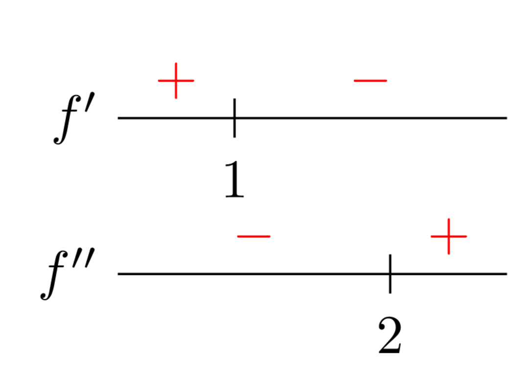
The last step before sketching is to make a sign chart, which I like to organize in the following way:

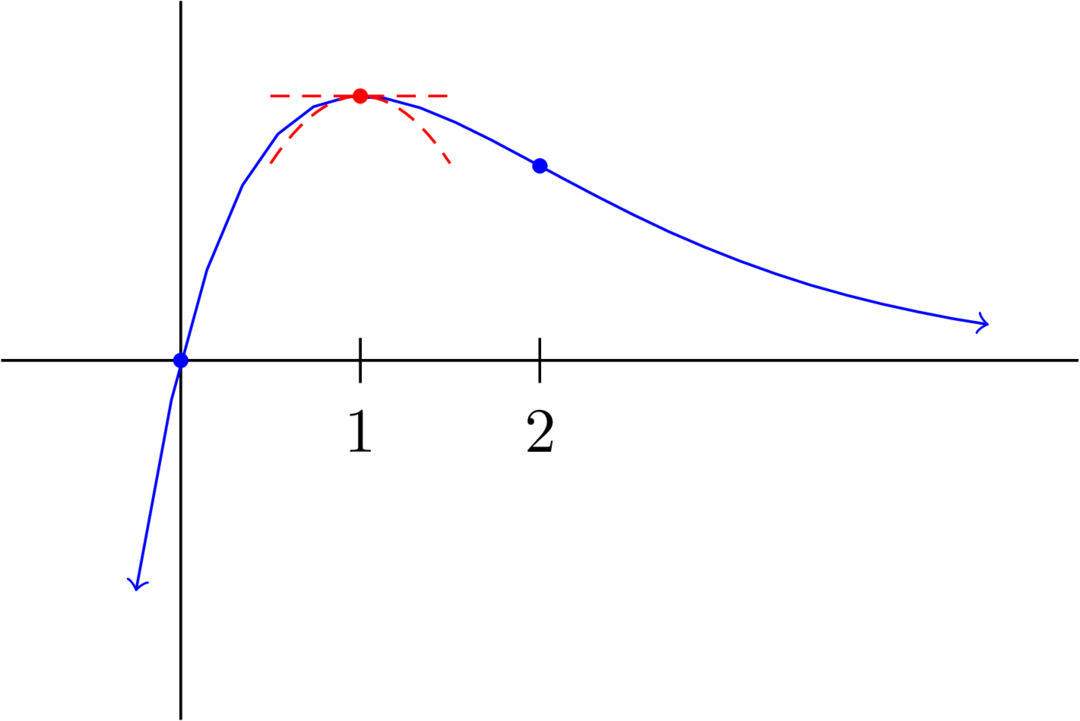
You should check the signs yourself. For example, if you plug in $x = 0$ , you get $f'\p{0} > 0$ , so $f'\p{x}$ is positive to the left of $1$ , and so on. From here, you just need to remember that $f''\p{x} > 0$ means $f$ is concave up and $f''\p{x} < 0$ is concave down, so you'll get this graph in the end:

The red line is to help you see where $f'\p{1} = 0$ shows up, and the red curve is to show you where $f''\p{1} < 0$ shows up. However, when you sketch these yourself, you don't need to draw anything that's in red here (unless it helps).

I recommend using Desmos to help you check your sketch after you try the problem out.

Example 8.

(7.3.60) Find the tangent line to $y = \ln\p{\sin{x}}$ at $x = \frac{\pi}{4}$ .

Solution.

The tangent line at $c = \frac{\pi}{4}$ needs to pass through the point $\p{c, y\p{c}}$ and have slope $y'\p{c}$ . So,

y\p{\frac{\pi}{4}} = \ln\frac{1}{\sqrt{2}} = \ln{2^{-1/2}} = -\frac{\ln{2}}{2}

and

y' = \cot{x} \implies y'\p{\frac{\pi}{4}} = 1,

so the equation of the line is given by

\begin{gathered} y - y\p{\frac{\pi}{4}} = f'\p{\frac{\pi}{4}}\p{x - \frac{\pi}{4}} \implies \boxed{y = x - \frac{\pi}{4} - \frac{\ln{2}}{2}}. \end{gathered}

Week 2 Discussion Notes

Table of Contents

Review of Exponentials and Logarithms

Proposition

Example 1.

Solution.

Exercise 1.

Theorem (change-of-base)

Proof.

Differentiation and Integration

Theorem

Proof.

Example 2.

Solution.

Example 3.

Solution.

Example 4.

Solution.

Logarithmic Differentiation

Example 5.

Solution.

Example 6.

Solution.

Homework

Example 7.

Solution.

Example 8.

Solution.