DENSITY CURVES

EXAMPLE 6.1

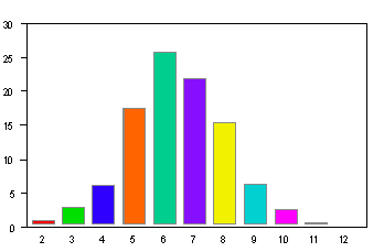
A reading test was given to 947 7^th graders and their equivalent reading grade level was determined.

class	%
2-2.9	.95
3-3.9	2.96
4-4.9	6.23
5-5.9	17.42
6-6.9	25.77
7-7.9	21.75
8-8.9	15.42
9-9.9	6.34
10-10.9	2.53
11-11.9	.53
12-12.9	.11

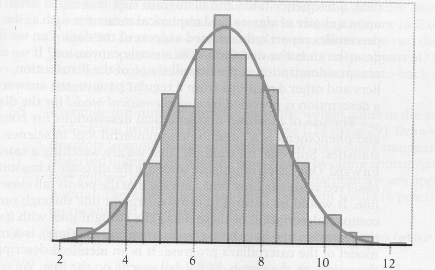
Suppose we try to approximate the histogram of the reading scores by passing a smooth curve through the tops of the rectangles. Let us make the vertical scale be proportions Using the full data set and a more refined grouping of the scores we get something like this:

Since histograms represent by areas, the proportion of students having reading scores between 4^th and 6^th grade would be the area in all the rectangles between these two limits. Observe that the area under the smooth curve between these same two limits approximately gives this area.

If we would examine the reading scores of other 7^th graders from other locations and make similar histograms and curves we would find that these graphs would all be slightly different but in essentials they would look very much the same.

This suggests the idea that one could make a mathematical model of reading scores that would give the essentials of the observed distribution of reading scores from wherever they are obtained in the following manner.

Suppose by means of some mathematical formula we could specify a curve (called a density curve)having the common characteristics of all the curves through histograms of reading scores. We could then say that the distribution of reading scores of 7^th graders between a and b (a<b) is the area under the curve between a and b. In this statement we are not referring to the reading scores of any particular set of 7^th graders but rather to some hypothetical collection of all possible 7^th graders.

THEORETICAL DISTRIBUTIONS

In general, to make a theoretical model of the distribution of some quantity of interest one does the following.

Specify a density curve for the theoretical quantity. Such a curve always on or above the horizontal axis and the total area under the curve is 1
Determine the proportion between a and b (a<b) by taking it to be the area under the curve between a and b.

It is useful to have a name for a quantity having a theoretical distribution. We call such a quantity a random variable. We usually denote random variables by capital letters such as X,Y,Z. We refer to the proportion of the values of a random variable X that fall between a and b as the probability that X is between a and b. We denote this as P(a<X<b). This probability is ,of course, just the area under the density curve between a and b. Values assumed by a random variable are denoted lower case letters. For example if the random variable is X then a particular value of X is denoted by x.

A Theoretical model is applied by assuming that the observed value of some real variable of interest is a just particular value of a random variable X.

Theoretical distributions have attributes just as do empirical distributions. For example, a theoretical distribution has a mean, a variance, a SD, a median, etc. These can be defined and calculated by means of the mathematical formula that specifies the density curve of the distribution. However, such computations are too advanced for this course.

The common notation for the mean of a theoretical distribution is (the Greek letter mu) and the standard notation for the SD of a theoretical distribution is (the Greek letter sigma).

If X is a random variable one often refers to some attribute of the distribution of

X, e.g. the mean, as an attribute of X. Thus, for example, we speak of the mean of X when we actually mean the mean of the distribution of X.

SOME BASIC RULES FOR PROBABILITIES.

P(X<a)=1-P(X>a)

If a<b then P(X<a or X>b)=P(X<a)+P(X>b)

Recall that the absolute value of a number x, denoted |x| is defined as |x|=x if x>0, |x|= -x if x<0, and |0|=0. Thus for example |5|=5 but |-5|=5.Thus |X|>a if ether X>a or -X>a. That is |X|>a if either X>a or X<-a. So P(|X|>a)=P(X>a)+P(X<-a)

P(|X|<a)=P(-a<X<a)